Automated Flower Classification using Deep CNNs
Introduction
This project develops and evaluates a deep convolutional neural network (CNN) for automated classification of flower species from images using the Oxford 102 Category Flower Dataset [3]. The network was implemented in PyTorch 2.2.2, trained on HPC resources (Viking cluster with H100 GPU), and achieved a final accuracy of 75.12% on the test set after extensive hyperparameter optimization.
Image classification represents a fundamental task in computer vision with applications spanning from medical image analysis [1] to botanical research [3]. Convolutional Neural Networks (CNNs) have emerged as the dominant approach for image classification since their breakthrough in 2012 [2].
Difficulties
The task of flower species classification presents unique challenges compared to simpler classification problems such as license plate recognition or manufacturing defect detection. The primary difficulties include:
- High intra-class variability: Same species appearing dramatically different under varying lighting conditions, growth stages, and environmental factors
- High inter-class similarity: Different species sharing similar visual characteristics (color, shape, texture patterns)
- Complex backgrounds: Natural environments with varying lighting and occlusion patterns
Applications
Automated flower classification has significant practical applications:
- Botanical research: Accelerating species identification processes [3]
- Plant breeding: Facilitating trait selection and genetic studies [4]
- Ecological conservation: Rapid identification and monitoring of invasive species [5]
- Agricultural optimization: Supporting crop management and yield prediction
Methodology
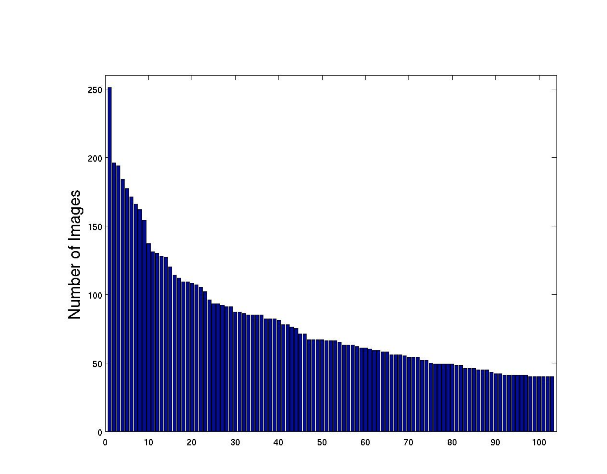
Dataset: Oxford 102 Category Flower Dataset
The Oxford 102 Category Flower Dataset contains images of flowers commonly occurring in the United Kingdom, with each class consisting of between 40 and 258 images. The dataset uses predefined splits:
- Training set: 12.5% (1,020 images)
- Validation set: 12.5% (1,020 images)
- Test set: 75% (6,149 images)
Each image was preprocessed by resizing to 224 × 224 pixels to match standard CNN input dimensions.
Data Augmentation Strategy
To address the limited training data and class imbalance issues [13], extensive data augmentation was implemented:
training_transform = transforms.Compose([
    transforms.Resize((256, 256)),
    transforms.RandomRotation(30),
    transforms.RandomHorizontalFlip(),
    transforms.RandomVerticalFlip(),
    transforms.ColorJitter(brightness=0.2, contrast=0.1,
                          saturation=0.1, hue=0.1),
    transforms.RandomAffine(degrees=20, translate=(0.1, 0.1),
                           scale=(0.8, 1.2)),
    transforms.RandomResizedCrop(224),
    transforms.ToTensor(),
    transforms.Normalize([0.485, 0.456, 0.406],
                        [0.229, 0.224, 0.225])
])
This augmentation strategy effectively doubled the training dataset size from 1,020 to 2,040 images, improving model generalization [12].
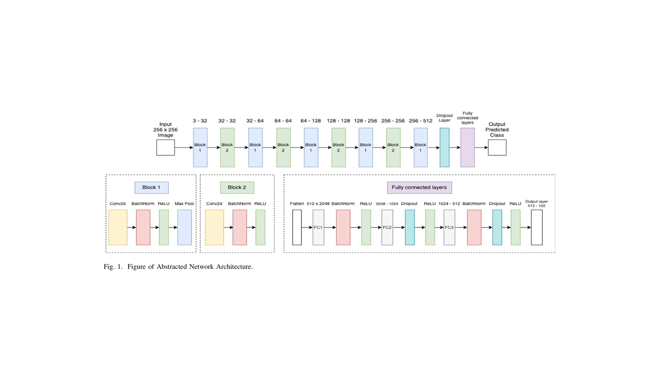
Network Architecture
The CNN architecture draws inspiration from VGG [8] and ResNet [9] designs, incorporating modern deep learning principles [6]:
Convolutional Stack (9 layers):
- Progressive filter expansion:
- Batch Normalization after each convolutional layer for training stability
- ReLU activation [7]:
- MaxPooling layers with kernels for spatial downsampling
- Dropout () for regularization
Fully Connected Classifier:
- Flattened feature maps: dimensions
- FC1: with BatchNorm1d and ReLU
- FC2: with Dropout (0.5) and ReLU
- FC3: with BatchNorm1d, Dropout (0.5), and ReLU
- Output: classes
Loss Function and Optimization
The model optimization employs cross-entropy loss [10], mathematically defined as:
where:
- — number of flower classes
- — ground truth one‑hot encoded label
- — predicted probability for class
The Adam optimizer [11] was selected for parameter updates:
where:
- Learning rate:
- Weight decay:
- Adam defaults:
Training Procedure
Hyperparameter Configuration:
| Parameter | Tested Values | Selected Value |
|---|---|---|
| Learning Rate | ([0.001, 0.0001, 0.00001]) | (0.0001) |
| Batch Size | ([8, 16, 32, 64]) | 8 (train), 64 (val/test) |
| Epochs | ([1, 1200]) | 1000 |
| Image Size | Various | (224 \times 224) |
Learning Rate Scheduling:
where and step size = 500 epochs.
The training process involved:
- Forward propagation through the 9-layer convolutional stack
- Feature extraction via global average pooling
- Classification through the 3-layer fully connected network
- Backpropagation using Adam optimizer for weight updates
Implementation Details
Hardware & Software:
- Cluster: Viking HPC (University of York)
- GPU: 1× NVIDIA H100 (80GB HBM3)
- Framework: PyTorch 2.2.2
- Training Time: 5.5 hours
- Language: Python 3.11
Results & Evaluation
Model Performance
The final trained model achieved a test accuracy of 75.12% across all 102 flower categories, representing significant improvement over the initial baseline accuracy of 4%.
Class-wise Performance Analysis
A detailed examination of the confusion matrix reveals that the model's performance varies significantly across different flower species, largely due to visual similarities and dataset imbalances.
Notably, flowers with similar appearances—such as certain lilies, orchids, and daisies—were often confused with one another, resulting in lower per-class accuracy. This trend highlights the limitations of the model when distinguishing between species with overlapping visual features, particularly in the presence of complex backgrounds or occlusions. The confusion matrix further indicates that classes with fewer training samples are more susceptible to misclassification, underscoring the importance of balanced datasets and targeted data augmentation for underrepresented categories.
Overall, while the model demonstrates strong performance on visually distinctive and well-represented classes, it struggles with species that are either underrepresented or visually similar to others. Future work could address these challenges by incorporating advanced augmentation techniques, leveraging transfer learning from larger botanical datasets, or integrating attention mechanisms to help the model focus on subtle discriminative features.
Conclusion & Future Work
This project successfully demonstrated the effectiveness of deep CNNs for automated flower species classification, achieving 75.12% accuracy on the challenging Oxford 102 dataset. The performance is particularly noteworthy given the small dataset size and high inter-class similarity.
Acknowledgments
This research was conducted using the Viking High-Performance Computing cluster provided by the University of York. I also thank the IT Services and Research IT team for computational support and infrastructure maintenance.
References
- [1]Q. Li, W. Cai, X. Wang, Y. Zhou, D. D. Feng, and M. Chen. "Medical Image Classification with Convolutional Neural Network". 2014.
- [2]L. Chen, S. Li, Q. Bai, J. Yang, S. Jiang, and Y. Miao. "Review of Image Classification Algorithms Based on Convolutional Neural Networks". 2021.
- [3]I. Gogul and V. S. Kumar. "Flower Species Recognition System using CNN and Transfer Learning". 2017.
- [4]
- [5]O. Iancu, K. Yang, H. Man, and T. Menard. "An Automated and Scalable ML Solution for Mapping Invasive Species". 2024.
- [6]
- [7]
- [8]K. Simonyan and A. Zisserman. "Very Deep Convolutional Networks for Large-Scale Image Recognition (VGG)". 2015.
- [9]
- [10]A. Mao, M. Mohri, and Y. Zhong. "Cross-Entropy Loss Functions: Theoretical Analysis and Applications". 2023.
- [11]
- [12]
- [13]U. F. Rahim and H. Mineno. "Data Augmentation Method for Strawberry Flower Detection in Non-structured Environment". 2020.
- [14]